Predicting Article Shares With Machine Learning In The Digital Marketing Industry

James Phoenix

Content creation is a time consuming and valuable activity. A marketers’ time for producing content is a precious resource and needs to be effectively optimized.

But is it possible for us to predict which articles will receive more shares than other articles by using machine learning and python?

Can we save our marketing teams from endlessly working on the wrong articles with the power of supervised AI?

Let’s find out… 😍

The Goal: To predict the number of shares an article will earn after being published for a minimum of 1 year on the internet.
James Phoenix

What Factors Will We Use?

BuzzSumo Metrics: Evergreen Score, Article Amplifiers and Total Shares (this will be the target variable that we will be predicting with our machine learning models).
Technical On-Page Metrics: (page load speed, no SSL/SSL etc).
On-Page Word Metrics: (word count, unique word count, number of sentences).
Unique, Impactful Words via TF-IDF Vectorization (every word is counted and assigned a score via the TF-IDF algorithm).
Off Page SEO Link Metrics: The number of backlinks pointing to a HTML page.

Topics Selected

To get some high quality article data, I used BuzzSumo pro and carefully selected the topics by keyword researching in Ahrefs.

The following 15 keywords had the highest monthly search volume and were chosen as topics:

Affiliate Marketing
Content Marketing
Copywriting
Display Advertising
Email Marketing
Growth Hacking
Influencer Marketing
Link Building
Marketing Automation
Performance Marketing
Podcast Marketing
Search Engine Marketing
Social Media Marketing
Video Marketing
Website Design

How We Will Evaluate Our Machine Models

The metrics for evaluating the machine models will be:

The R² Score from cross validated data. This is otherwise known as the proportion of variance in the dependent variable (Total Shares) that can be predicted from the other independent variables (Sentence length, number of links etc.).
The error function: The residual sum of squares was the chosen error function and is calculated in the following manner:

Simply put, all of the blue dots on the graph below are the real total shares from Buzzsumo data. For every data point the red line shows the distance (error) between the actual value and the predicted value.

This is then summed for every point, so if there was no difference (zero values overall) between the actual and predicted values, then we would always be able to predict the total shares of an article without any error.

Want to improve your data skills?

See the best data engineering & data science books

Shop Now

Executive Summary:

Using a variety of regression models, the highest predictive score achieved was an 0.85 R² score from 100 random forest estimators as an ensemble method. Taking the logarithm + 1 of our target variable (‘Total Shares’) allowed for the model score to improve from 0.35 R² to 0.85 R² .

The most important coefficients that impact the sharability of an article are:

Evergreen Score
Does the article have article amplifiers? (True / False)
Does The Article Page Have Referring Domains (True / False)

Negative coefficients that decreased the chance of an article being shared are:

Number of Linking Pages
No SSL Encryption (True / False)
Meta Description Length

TLDR; Key Takeaways ❤️

Focus on producing more evergreen content.
Prioritise creating how to guides over infographics and list posts.
Leverage relationships with key influencers to increase the number of article shares.
Focus on long-form content as this was a positive coefficient in the LassoCV model (higher number of sentences).

The Machine Learning Process

1. The Data Sources

15 topics were downloaded from BuzzSumo’s pro plan (a 3 month snapshot was taken):

30,000 Article URL’s were collected from BuzzSumo’s Pro Plan.
A custom, multi-threaded Python web crawler was created for extracting 61 metrics from every HTML web page.
Google’s Page Speed API was utilised to extract page speed metrics for every article.

2. Data Collection & Pre-Processing

Cleaning The BuzzSumo Data + Identifying A Target Variable

Our target variable is defined as total_shares in column D, so now let’s remove any redundant columns:

Thumbnail
Video
twitter_shares, pinterest_shares, total_reddit_engagement (These metrics are directly correlated with our target variable and therefore we cannot use them)

Creating Dummy Columns For The Discrete (Categorical) Variables

Additionally I decided to create dummy variables (true / false variables) on all the non-numerical columns to ensure that these can be used as features within the modelling stage. For example we can tag every article with its specific article_type.

Creating A Web Python Web Scraper

Then I created a data structure for the Python Web Crawler to capture a range of features from the HTML web page. This included article information, NLP features, readability scores, meta data and technical features such as whether the web page was secure or not (HTTPS vs HTTP).

data dictionary example for web scraping

Now that we have an ideal data structure for capturing additional features, it’s essential that we can extract only main body content of an article/html page. For this I used the Python library Newspaper3k!

I successfully obtained the main body content for 15,000 URL’s out of the original 30,000 URLS.

Google Page Speed Insights Data

We can further enrich the dataset with web page speed metrics from Google. I collected the content meaningful paint + time to interactive web page speed metrics for the remaining 15,000 URL’s. These were then merged with the existing data (BuzzSumo + Web Crawled Data) with again, the URL acting as the common key.

So now we have BuzzSumo data, Web Crawled Data and Page Speed Metrics within the same dataset! 😀🚀

Why Combine Multiple Data sets?

By blending together several data sources we are able to gather significantly more features for our machine learning models.

We are trying to increase our chances of finding discrete or continuous variables which are either strongly positively/negatively correlated with our target variable (total article shares).

However if there are too many features this can quickly lead to:

Over-fitting the training data – Our models start fitting noise and will have higher training scores, yet lower cross validation and test scores (this means that our model would generalize less to unseen data).
Also models such as the random-forest regressor or a decision tree regressor can struggle to achieve significant results when the feature space (number of variables) has too many dimensions.

3. Exploratory Data Analysis (EDA)

Before we start modelling the data, let’s explore the relationships between all of our variables and look for any immediate insight/trends.

Correlations Between The X-Predictor Matrix & The Target Variable (y)

On the left we can see what variables are most positively correlated with our target variable.
- Evergreen Score.
- Number of Linking Domains.
- Whether the Article Has An Article Amplifier.
On the right, there were not many strong negative correlations.

The Target Variable – (Total Article Shares)

As you can see in the above graph the target variable is highly skewed and is not normally distributed. This means that the majority of articles only receive a small number of shares. Also, it appears our target variable is likely to be from an exponential distribution.

From my initial, poor results with simpler machine learning models (linear regression, lassoCV and ridgeCV), it was evident that the target variable was struggling to form a strong linear relationship with the predictor matrix (the other independent variables).

Therefore I decided to apply a np.log(+1) transformation to the target variable, which looks like this:

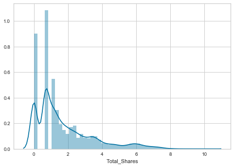
Although the distribution is still positively skewed, it certainly has less of an exponential shape.

Some easy insights…

Interestingly, the most popular topics were: Search Engine Marketing, Growth Marketing & Social Media Marketing.

Articles tagged with “how to articles” & “why post” on average received the most amount of shares and were followed by infographics and list articles.

Therefore the insight that we can gain is that people reading digital marketing topics share on average content which is:

Educational – (how to articles)
Visual – (infographic articles)
Easily digestible – (list articles)

4. Machine Learning Model Results Summary

The most impactful model was an Ada Boosted ensemble method with 5 x RandomForest’s (100 estimators each) as the base estimator.
Adding the web page speed data from Google Page Speed Insights, increased the mean cross validation score on our best model by ~ 5%.

Okay that’s great but let’s look at some simpler models and see what we can learn from them (linear regression):

Modelling – LassoCV

The positive coefficients in the above example are for a linear regression model. This model shows us that as the sentence length increases by 1, the logarithm value of the total article shares increases by 0.1.

Equally so, the model coefficients describe that if the article Has_Referring_Domains variable is true then the logarithm value of total article shares will increase by 0.735.

The left graph shows y (log shares) vs y^ (predicted log shares).

The right graph shows that after 4000 data points, we start to achieve consistent results with our regression model. This means we only need to obtain 4000 samples before attempting any further modelling tasks in the future.

Modelling – Decision Tree Regressor

In order to simply look at the feature importances, I decided to use a max -depth 5 decision tree instead of a random forest.

Firstly the evergreen score is a calculated metric within BuzzSumo and is meant to dictate ‘how evergreen’ a piece of content is.
The number of linking domains is how many do-follow backlinks are pointing at the article.

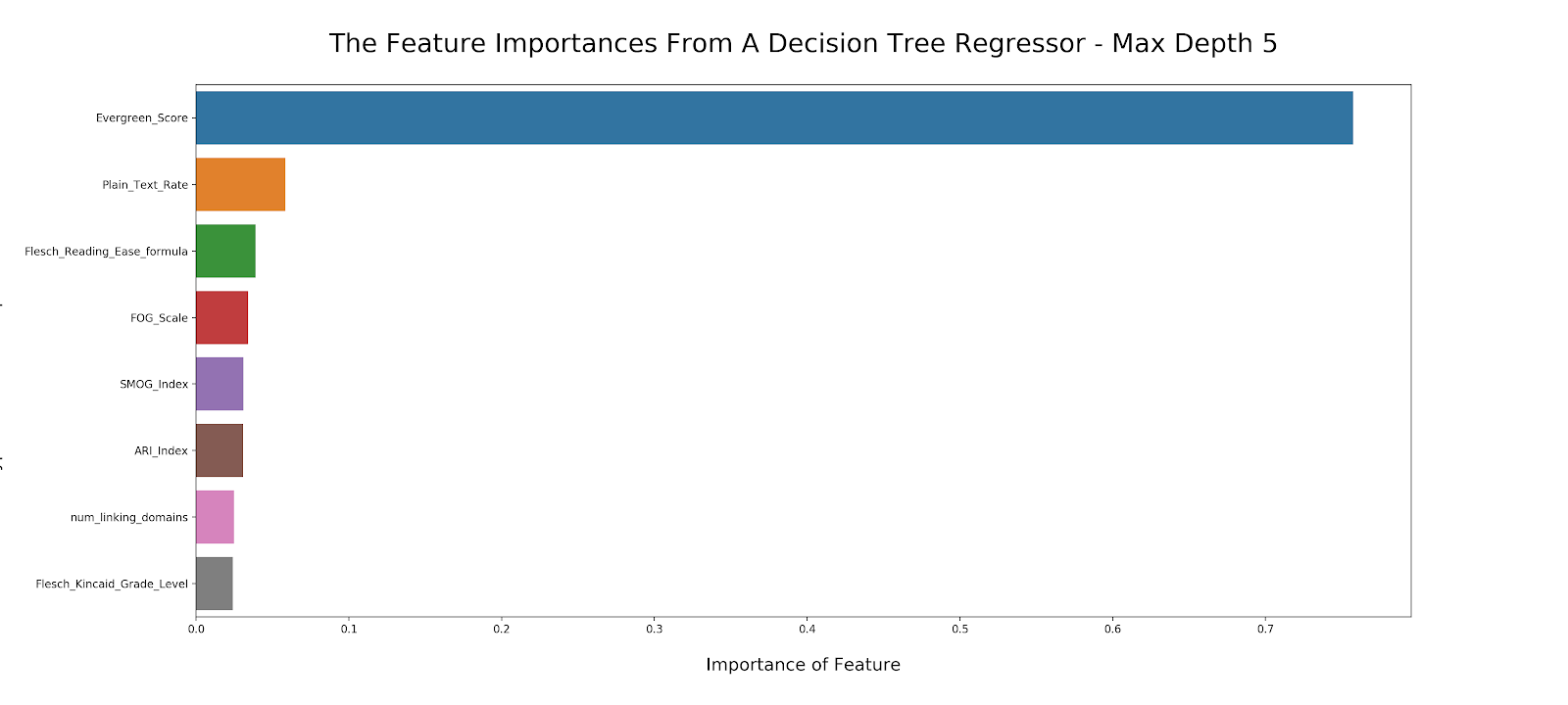
The most important features in determining the decision boundaries for the logarithm value of y are:

Evergreen Score
The Number of Linking Domains
Readability Scores
Plain_Text_Rate

The Title Tag Length Is More Important Than You Think…

Additionally for articles that had more than 0.5 article amplifiers and a higher evergreen score than 0.155. 5852 out of 12594 samples were divided by the Title_Tag_Length (see graph above).

Now we can infer that:

Having a title_tag_length greater than 79.5 characters predicts less article shares.
Also if the title_tag_length is less than 45.5 characters also predicts less article shares.

This makes sense because we want a catchy, strong headline that entices someone to click and read the article.
However if the article headline is too long then it will cause the title to be truncated within the Google SERPS (search engine results pages) which often leads to a lower click through rate for the article.

So for digital marketing content, keep your title tags between these two ranges for optimal results.

An example of title tag truncation can be seen below:

Key Takeaways ❤️

Focus on producing more evergreen content.
Prioritise creating how to guides over infographics and list posts.
Focus on long-form content as this was a positive coefficient in the LassoCV model (higher number of sentences).
Leverage relationships with key influencers to increase your article shares.

Additionally soon I will be releasing a live, open version of this model which will be accessible via a Flask implementation. For more information regarding this project feel free to visit my Github page. 👍

Challenges

30,000 articles were downloaded, however I was only able to obtain the article text data for 15,000 URL’s, this was simply because the type of Python package that I was using wasn’t able to extract the main body content for half of the data.
Working with text data naturally creates sparse matrices, this can be problematic because it drastically increases the dimensionality of the feature space. In order to combat this challenge, a custom standard_scaler and TFID_vectorizer class were created in sci-kit learn for optimising the pipelines and grid_search process.
The target variable ‘Total Shares’ was not normally distributed and was exponentially distributed. From taking the logarithm and adding +1 to all values we were able to create a better, more linear relationship between our predictor features and our target variable.
Some of the articles had 404’ing pages, therefore whilst web scraping excessive exception handling was required to ensure that all of the features gathered were aligned to the correct URL’s.
The variables which our best predictors were only available via BuzzSumo, which means our predictions currently rely on a 3rd party tool.

Risks / Limitations

The sample that we chose was 1 year old, this was selected to remove any bias of an article not being online enough to receive a significant part of it’s online shares. However this type of sample could lead to bias within the model’s predictions. Therefore it would be advisable to study the natural share cycle of article’s and the share velocity from when an article is originally published until it reaches a certain level of maturity.

Omission Bias: Only selecting mature websites will almost certainly impact the ‘shareability’ – this means that the model could potentially be over-/under-estimating the effects of certain factors because this factor is not properly controlled for or included in the model.

The Newspaper3k python library was only able to collect 15,000 articles from the original 30k data set. Therefore the remaining URL’s had to be discarded.

Assumptions

Taking a sample of articles for a 3 month people might not be a representative sample, furthermore seasonality might have an influential factor on how article’s are shared across different topics.
There is a lagged component that hasn’t been included in the model. (i.e. article’s receive shares over a series of months. Not as a given snapshot).

By not taking into account the time component, it can lead to spurious relationships (i.e. if x and y variables increase over time the model could tell us that there is a strong relationship but actually both could be independent and an another variable could be driving the relationship as a confounding factor.

Next Steps

Perform a sentiment analysis over time.
To model the data on a neural network as from having to apply a logarithm to the target variable we can clearly see that the relationship is less linear with the original target variable scale. A neural network might be more able to model the non-linear relationships between the predictor matrix and the target variable.
Using a time-series model with the original features as additional features (exogenous features).
It would also be good idea to track articles / topics for several months or years. This would allow us to perform time series analysis on individual topics.

Conclusion

Ada Boosted RandomForestRegressor was the best performing model.
Taking the logarithm of the target variable (Total_‘Article_Shares’) helped to improve the model scores by creating a more linear relationship between our predictor features and ‘Total_Article_Shares’.